ASRS for distribution centers is usually sold on a device number: a shuttle travel speed, a crane cycle, a lift acceleration. None of those numbers tells a distribution center whether it will clear its carrier cut-off next November. The rate that matters is a system rate, meaning pallets per hour that complete the full loop from receiving through storage to a pick face and back, sustained across a shift, under the order profile the site actually runs. In most distribution center designs the binding constraint is not the storage and retrieval machine. It is the number of vertical transfer points, the capacity of the stations being served, and the dispatch logic that sequences work across both.
What Throughput at Scale Means in a Distribution Center
A distribution center differs from a production warehouse in one way that shapes every throughput calculation. Inbound is often pallet-uniform and predictable, while outbound is layer-picked, case-picked or each-picked against a carrier cut-off, so demand arrives in waves rather than a smooth line. The putaway mix and the retrieval mix are therefore different, dual-cycle opportunities are fewer than a production site enjoys, and the peak hour carries most of the design risk.
Four distinct rates get mixed together during procurement, and separating them early prevents a painful argument later.
| Rate | What it describes | Where it belongs in the project |
|---|---|---|
| Peak hour rate | Highest sustained 60-minute window in the year, set by cut-off times and wave release | Sizing the fleet, the transfer units and the station count |
| Sustained shift rate | Completed moves per hour across a full operating shift at a defined SKU mix | The contractual acceptance figure |
| Device rate | One vehicle or one machine working without contention | An input to the cycle-time calculation |
| Retrieval latency | Time from a release to a pallet arriving at the station | Wave planning and station staffing |
The fourth row is the one buyers forget. A system can hit its hourly total while still breaking wave picking, because the first pallet of a wave arrives forty minutes after release. Latency and hourly rate are separate commitments and both need a number in the specification.
There is also a geometry tradeoff that distribution centers feel more than most. Deeper lanes and denser racking raise storage density per square metre, but they increase honeycombing and extend the average travel distance, because more pallets sit behind others that must be moved first. In a site whose SKUs turn quickly, that extra travel can consume more system rate than the rack saves in floor area. Density and throughput are both legitimate goals, and the layout has to state which one yields when they conflict.
Where ASRS Throughput Is Actually Lost
Throughput is lost at the points where every pallet must pass. A storage system contains two kinds of element. Parallel elements add rate as you add units, which is what a shuttle fleet does. Serial elements do not, because every pallet in the loop has to use the same device, and that device sets a ceiling the fleet cannot lift.
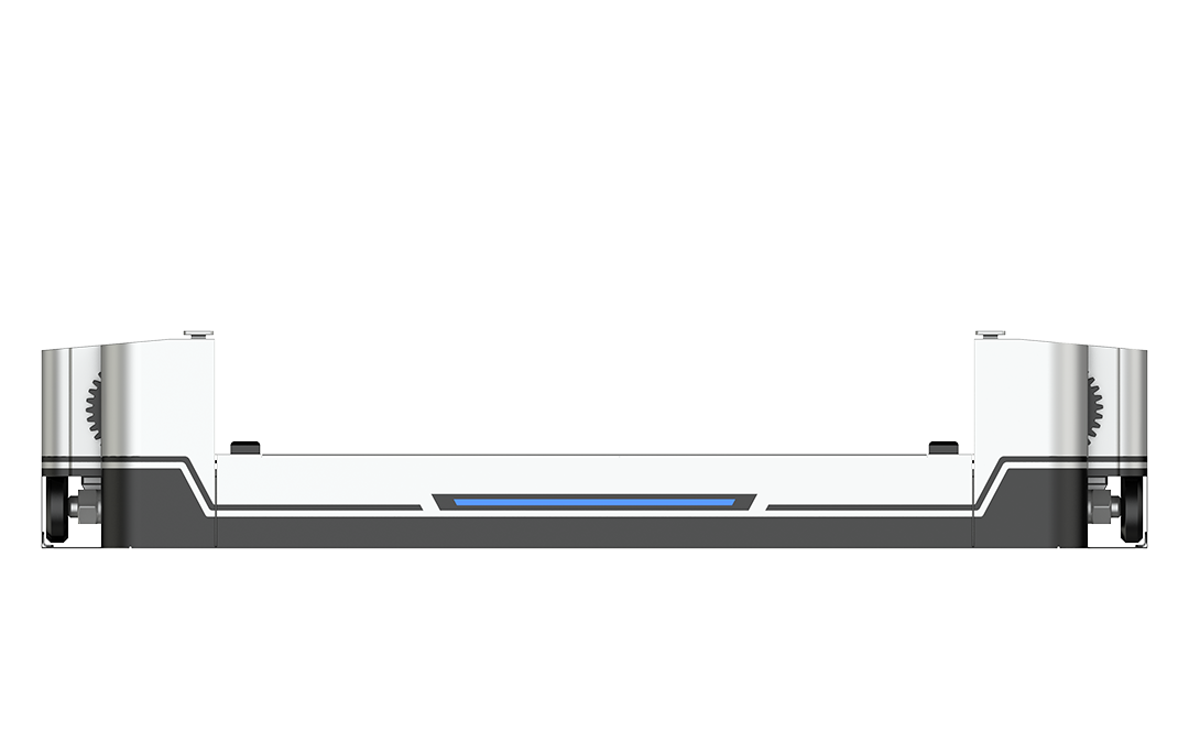
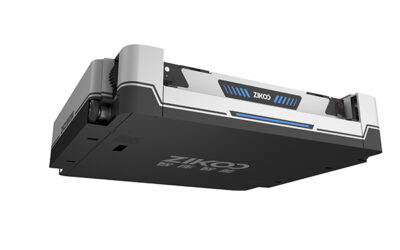
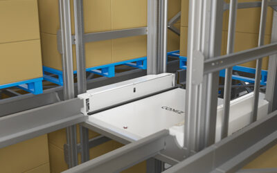
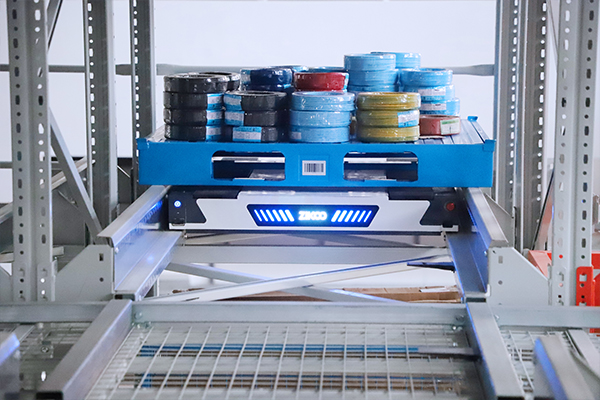
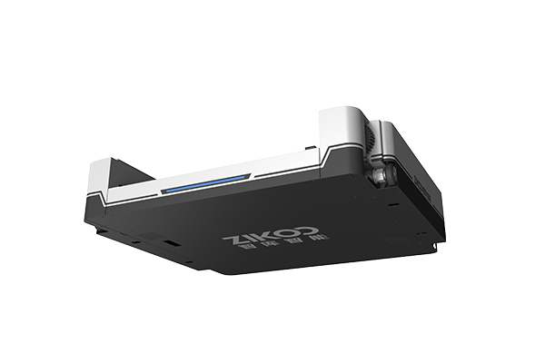
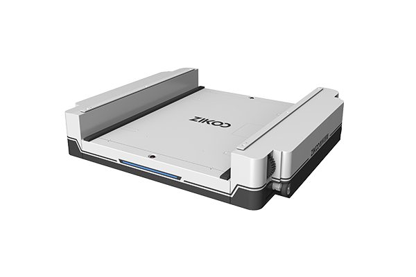
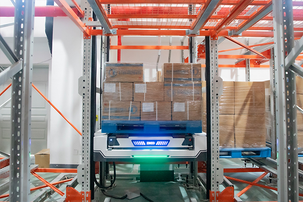
The vertical transfer point is the classic serial element. Published specifications for the R-bot four-way shuttle and the H-bot vertical transfer unit illustrate the split clearly. The shuttle runs at 1.6 m/s empty and 1.2 m/s loaded with a body only 125 mm thick, which lets it work inside dense rack levels. The transfer unit positions to plus or minus 1 mm at 1 m/s empty and 0.5 m/s loaded with acceleration of 1 m/s² empty and 0.3 m/s² loaded, and it occupies a single storage location rather than a dedicated shaft. The shuttle’s contribution multiplies with fleet size. The transfer unit’s cycle does not, because every level change passes through the same device. In a layout with one transfer point per zone, that zone’s rate is capped by the transfer unit no matter how many shuttles are added to the aisle.
| Constraint | Why it caps system rate | What to check in the design |
|---|---|---|
| Vertical transfer points | Serial device, every level change passes through it | Transfer count, acceleration profile, redundancy, service access |
| Station induction capacity | People and lift tables set the pace at the pick face | Pallets or lines per hour per station, replenishment policy, buffer depth |
| Conveyor merges and scanners | Single-file handoff creates queueing upstream of the merge | Merge logic, bypass lanes, read rate, recirculation rules |
| Dispatch and task sequencing | Idle travel and single-cycle operation waste fleet time | Dual-cycle share, pre-positioning rules, deadlock handling |
| Charging and battery windows | Vehicles are unavailable while charging | Opportunity charging policy, swap strategy, charge ratio at peak |
| Aisle and lane geometry | Deep lanes raise honeycombing and average travel | Lane depth against the velocity distribution of the SKU base |
The practical consequence is uncomfortable for anyone comparing quotations on vehicle count. Adding shuttles to a system with a saturated transfer point adds capital cost and aisle congestion, not throughput. Before the fleet size is fixed, the design should identify which element saturates first at the target rate, and then confirm that this element has the margin to absorb a peak hour and a maintenance outage.
Shuttle-Based ASRS Versus Unit-Load Stacker Cranes
The two architectures solve the same problem with different scaling levers, and both are credible at distribution center scale.
A unit-load stacker crane puts one machine in each aisle. Its cycle is deterministic and easy to model, it reaches very high bays that shuttle systems cannot, and its per-aisle behaviour is predictable. Its constraint is that rate per aisle is fixed by one machine, and an aisle with a crane out of service is an aisle with no capacity.
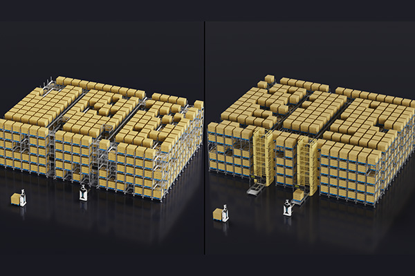
A shuttle-based ASRS puts multiple vehicles into the same level and aisle structure. Rate scales with the fleet rather than with the aisle count, a single stopped vehicle is absorbed by the others, and the rack can be built deep. The cost of that flexibility is dependency on transfer points and on dispatch software that prevents vehicles from blocking each other in shared travel paths.
| Dimension | Shuttle-based ASRS | Unit-load stacker crane | Evidence status |
|---|---|---|---|
| Rate scaling | Adds vehicles into existing levels | One machine per aisle, fixed ceiling | Architecture-level, checkable in design documents |
| Redundancy | Fleet absorbs one stopped vehicle | Aisle loses capacity with the crane | Depends on maintenance and spares strategy |
| Height | Bounded by transfer design and rack structure | Reaches very tall single and double deep bays | Confirm against the actual building and mast height |
| Density | High with deep lanes across many levels | High with single or double deep rack | Both are dense, compare aisle count and honeycombing |
| Transfer dependency | Requires lifts or satellites | Travels vertically on its own mast | Design consequence, not a performance claim |
| Congestion risk | Higher, needs traffic and deadlock rules | Lower within an aisle | Verified in simulation or reference runs, not in brochures |
Neither column wins in general. A tall building with a narrow SKU base and a moderate rate is well served by a crane, and the simpler control problem is worth real money. A twelve to twenty-four metre building with a wide SKU base and a rate that must rise with volume usually needs the scaling lever that a shuttle fleet provides, provided the transfer and station side is designed to match. The mistake is choosing the vehicle architecture first and discovering the serial constraint afterwards.
Dense storage only returns its throughput when the vehicle architecture matches the rack structure and the order profile behind it. <Smart Storage Revolution: Comprehensive Overview of Four-Way Shuttle Systems for Automatic 3D Warehouses> covers how four-way shuttle systems are configured for automatic 3D warehouses.
Sizing Shuttles, Lifts and Stations for a Target Rate
Fleet sizing is arithmetic once the cycle time and the utilization factor are defined, and it is guesswork when they are not. The order below matters, because the parallel side is estimated first only to show how little it constrains the answer.
Estimate the vehicle side
The vehicle requirement follows a single relationship. Required vehicles equals the target rate divided by the effective hourly rate of one vehicle, where the effective rate is 3600 divided by the average cycle time in seconds, multiplied by a utilization factor. The cycle time must come from a declared convention, such as an average combined cycle over a randomized location pattern, because a best-case single cycle flatters the result. The utilization factor covers contention, charging and blocked travel, and it should come from a simulation or a reference site with a comparable layout, not from an assumption.
Check the serial side separately
A transfer unit’s rate is 3600 divided by its cycle time in seconds. That number is fixed. Compare it against the share of moves that must cross a level, and the difference between the two figures is the margin the design actually has.
The following numbers are illustrative and chosen so the arithmetic is easy to follow. They are not a quotation and not a project result. Take a target of 240 pallet moves per hour sustained. An average combined cycle of 90 seconds gives 40 moves per hour per vehicle at theoretical pace. A utilization factor of 0.75 brings that to 30, so the fleet requirement is eight shuttles. On the serial side, a transfer cycle of 45 seconds including positioning and handshake gives 80 transfers per hour per unit at full utilization. If 70 percent of moves cross a level, lift demand is 168 transfers per hour, which is 2.1 units at theoretical pace. Three units leave almost no margin for a peak hour or an outage, and four leave a defensible one.
The lesson from that arithmetic is not the number eight. It is that the shuttle count has a comfortable margin while the transfer count is the decision with the least slack, and it is the decision a buyer usually spends the least time on.
How Software Decides Whether the Hardware Rate Is Reachable
Installed capacity and realized capacity diverge in the control layer. The warehouse management layer owns inventory and orders, the execution layer owns flow and prioritization, and the control layer owns device dispatch and traffic. In systems that also run mobile robots, a robot control layer allocates tasks to those units. The rate the site experiences is produced by whichever layer makes the next-task decision.
Five levers in that decision matter more than most hardware upgrades.
- Task interleaving. A vehicle that retrieves and then performs a putaway on the return leg does nearly twice the work of one that returns empty. The order pool has to be presented in a way that makes pairing possible.
- Pre-positioning. Moving fast-moving pallets closer to the stations during low-demand windows shortens the peak cycle before the peak starts.
- Slotting refresh. Velocity-based slotting set once at go-live decays within a season. It needs a scheduled review against actual order history.
- Delivery pacing. Releasing a wave in one burst fills the conveyor and the station buffer, and the queue time is then counted against the storage system even though the storage system did not cause it.
- Exception handling. A single unreadable label or a pallet outside tolerance should not stall a loop, and the recovery rule should be written before go-live rather than discovered during it.
A dispatch policy that sends every idle vehicle to the farthest available task will underperform one that reserves nearby work, and the difference appears as a shortfall that looks like a hardware problem.
Dispatch rules and slotting decisions determine how much of the installed fleet capacity a distribution center actually uses each hour. <Software-Driven Hardware: Six-Way Shuttle Maximizes Warehouse Efficiency> covers how software control shapes six-way shuttle system efficiency.
Peak Season, Frozen Zones and Multi-Shift Duty
Conditions change the achievable rate, and they should be priced into the design rather than discovered in operation.
In a frozen zone, battery capacity and charge acceptance both fall with temperature, so the vehicle that meets the target in ambient conditions needs either a dedicated low-temperature pack, an insulated or heated charging position, or a shorter duty cycle between charges. Published cold-chain configurations show the pattern: dedicated low-temperature batteries with six to eight hours of continuous operation, a charging port designed for automatic connection at low temperature, and conformal coating on the control boards for high-humidity environments. Standard models are rated to minus 15 degrees Celsius while transfer units in the same family are rated from minus 25 to 45 degrees Celsius, which is a reminder that the coldest rated component in the loop is not necessarily the vehicle. Condensation on transfer between zones also affects pallet stability and label readability, and both cost time at the station.
Peak season needs a separate answer from average season. Pre-building inventory in position, deferring non-urgent putaway, adding station labour and holding a manual overflow path are all cheaper than buying capacity that idles for ten months. What matters is that the peak plan exists and that the control layer can execute it, rather than being improvised in the first week of December.
Redundancy belongs in the same conversation. A design with one transfer unit per zone has no degraded mode, only a stop. A design with a spare transfer point or a cross-zone route can run at reduced rate through maintenance, and that reduced rate should be stated in the contract.
Cold store throughput depends on battery behaviour, charging access and service routines as much as on storage density. <Smart Cold Chain Era: Six-Way Shuttle System Redefines Storage Efficiency with Maximum Density> covers how a six-way shuttle system is applied to cold chain storage density.
What to Specify and How to Test It Before You Sign
A throughput clause is only as good as the definitions behind it. Four definitions carry most of the weight: what counts as a completed move, over what window it is measured, at what SKU mix and inbound to outbound split, and with which equipment in service. A move that counts a putaway and a retrieval separately produces a different number from one that counts a combined cycle once, and the gap is large enough to decide a contract.
The wording matters just as much as the definitions. Consider the difference between these two lines.
Reject this line: the system shall handle 300 pallets per hour.
Replace it with: the system shall sustain not fewer than the agreed target of completed pallet moves per hour, measured at the control layer over any continuous four-hour window within a twelve-hour shift, at the SKU mix and inbound to outbound split in the approved appendix, with all transfer units in service; with one transfer unit out of service the system shall sustain not less than 75 percent of that figure, and the definition of a completed move, the measurement basis and the data source shall be agreed before the factory acceptance test.
That revision is longer, and it is the only version that can be tested without an argument. It also forces the two sides to agree on which equipment counts as in service, which is where most disputes actually start.
Different kinds of throughput evidence prove different things, and the table below is worth carrying into a supplier meeting.
| Record | Method context | Responsible use | Do not infer |
|---|---|---|---|
| A pallets per hour figure in a brochure | Usually one vehicle, one cycle, no contention | Screening whether an architecture class could plausibly reach the target | That the installed system will deliver it on your SKU mix |
| A supplier simulation | Built on data you supplied, with stated assumptions | Testing whether the assumptions match your order profile | That the real system matches the model without an agreed tolerance |
| A reference site visit | One shift, one date, conditions you did not control | Sense-checking flow patterns and staffing levels | A measured sustained rate, since the mix differs from yours |
| A factory acceptance test | Defined move, defined window, defined equipment state | A contractual benchmark for that configuration | That the rate holds in peak season with a wider SKU base |
| A published vehicle specification | Single-unit travel speed, empty or loaded | Input to a cycle-time calculation | Any system throughput figure, which depends on transfers, stations and dispatch |
Site conditions decide as much as any of these records. Pallet quality, overhang, damaged corner posts, load stability and unusual load shapes all affect whether a system runs at its calculated rate, and heavy or awkward loads in an energy sector distribution center need their own check rather than an assumption that a standard pallet definition covers them.
Send Your Peak-Hour Profile Before You Commit to a Layout
The most useful next step is not a request for a quotation. It is a short exchange of data that identifies which element will saturate first in your building. Send the peak hour rate and the sustained shift rate you need to hit, the inbound to outbound split, the pallet dimensions and weights including the badly stacked ones, the temperature zones, the SKU velocity curve, and the building height and column grid. Each of those changes the answer: the split sets dual-cycle potential, the velocity curve sets lane depth, and the column grid sets aisle count.
Zikoo can review that profile against shuttle, transfer and software configurations and tell you where the constraint is likely to land. It will not replace a site survey, a load test or a validated simulation, and it should not be treated as a commitment to a specific rate in your building. Contact the team at info@zikoo-int.com or call (+86)-19941778955 with the profile attached.
FAQ
How many pallet moves per hour can an ASRS handle in a distribution center?
There is no honest single number, because the system rate is set by the slowest serial element in the loop rather than by the vehicles. A well designed shuttle system can be scaled to a high rate by adding vehicles, but its transfer points, station capacity and dispatch logic cap what the site actually experiences. Ask instead for the transfer cycle, the station rate and the cycle-time convention behind any quoted figure, then check that the arithmetic closes.
Is shuttle-based ASRS faster than a stacker crane system?
Not in every case. A stacker crane gives one machine per aisle, so its per-aisle rate is fixed and an outage removes an aisle. A shuttle system adds rate by adding vehicles into the same level, so it scales further, provided the transfer points and stations keep pace. In a very tall building with a narrow SKU base and a modest rate, a crane is often the simpler and more predictable choice.
What usually causes a throughput shortfall after go-live?
Four causes account for most of the gap. The measured move was defined differently from the contractual one, the SKU mix shifted towards slower or bulkier items, the slotting was never refreshed after commissioning, or the transfer and station side was sized on an average hour rather than the peak. Only the last of these requires capital to fix, which is why it is worth resolving before the layout is frozen.
Can an ASRS handle peak season surges?
Yes, if the peak was designed in rather than assumed away. Pre-building inventory in position, deferring non-urgent putaway, adding station labour and keeping a manual overflow path are usually cheaper than buying capacity that idles for most of the year. What matters is that the control layer can execute those measures on command, and that a degraded mode with one transfer unit out of service still clears the cut-off.
Do we need a simulation before buying at this scale?
For a distribution center with a real peak, yes, but the value depends on the assumptions being visible and testable. Require the model to state its cycle-time convention, its SKU mix, its contention and charging assumptions, and the tolerance it claims. A simulation with hidden assumptions produces a confident number that cannot be defended at acceptance, which is worse than an agreed calculation you can check by hand.
If you’re interested, check out these related articles:
Software-Driven Hardware: Six-Way Shuttle Maximizes Warehouse Efficiency
Stacker Crane vs Four-Way Shuttle: Which Fits Your ASRS Warehouse Best
Six-Way Shuttle Powers Dense Storage: Breaking Space Limitations
Six-Way Shuttle Unlocks the Era of True 3D Intelligent Warehousing
Standardization Empowers Global Delivery: Zikoo Robotics Six-Way Shuttle Expands Overseas